Through college I was getting bored of my courses as I learned about logical operational rules of the road. Then came my first Python course and I started to see the countless possibilities and power of data. This was my very first Python project result and it happens to include penguin data:
https://TMITLT.com/projects/penguin-weights
I know it is impressive how great my graphic design skills were/are – please do not solicit art. I am not taking requests at the moment.
More info on this project:
Data source: Palmer’s Penguins
Table of Contents
The Penguin Python
First I import the data and save it in a variable and view it
import pandas as pd
data = pd.read_csv('penguins_size.csv')
datadata['sex'].unique()array(['MALE', 'FEMALE', nan, '.'], dtype=object)
I need to clean the data. Notably, there are NAs and the sex column has “.” as an entry. After the code is cleaned I can check the shape of the data to make sure I still have enough entries less to work with.
data = data.dropna()
data = data.loc[~(data['sex'] == ".")]
data.shape
data['sex'].unique()
(333, 7)
array(['MALE', 'FEMALE'], dtype=object)
Data Review
import matplotlib.pyplot as plt

plt.hist(data['body_mass_g'])

plt.xlabel("Weight")

plt.ylabel("Count")

plt.title("Histogram of Body Mass")
With 333 data entries I can continue. Now I split those entries into train and test data. I will make 80% of the data the train data.
train_data = data.sample(frac = 0.8, random_state = 0)
test_data = data.drop(train_data.index)
Now that I have the data I want to work with I can visualize my Independent and Dependent variables seperately to check if a relationship is apparent
plt.scatter(train_data["culmen_depth_mm"],train_data["body_mass_g"])
plt.xlabel("culmen_depth_mm")
plt.ylabel("body_mass_g")
plt.title("body_mass_g vs. culmen_depth_mm")
It looks like there is a positive relationship but the division in the data shows we likely also need some categorical variable to explain the deviation.
plt.scatter(train_data["flipper_length_mm"],train_data["body_mass_g"])
plt.xlabel("flipper_length_mm")
plt.ylabel("body_mass_g")
plt.title("body_mass_g vs. flipper_length_mm")
from sklearn.preprocessing import PolynomialFeatures
from sklearn.linear_model import LinearRegression
from sklearn.model_selection import cross_val_score
import numpy as np
from numpy import mean

#Define predictor and response variables.
x = np.array(train_data['flipper_length_mm']).reshape(-1,1)
y = np.array(train_data['body_mass_g'])

degree = []
cv_errors = []
for i in range(1,10):
  #i represents the degree of the polynomial. This code checks i = 1,2,...,5.
  degree.append(i)

  #Specify the type of model.
  poly_x = PolynomialFeatures(degree=i, include_bias = False)
  xp = poly_x.fit_transform(x)
  model = LinearRegression()

  #Implement leave-one-out cross-validation.
  scores = cross_val_score(model, xp, y, cv=5, scoring = 'neg_mean_squared_error')
  cv_errors.append(-mean(scores))
  print('Degree of polynomial: ', i, ' Cross-validation error: ', -mean(scores))
Degree of polynomial: 1 Cross-validation error: 162417.08191747055 Degree of polynomial: 2 Cross-validation error: 151644.6910167652 Degree of polynomial: 3 Cross-validation error: 146514.54782842658 Degree of polynomial: 4 Cross-validation error: 146353.33382326312 Degree of polynomial: 5 Cross-validation error: 146337.72330430784 Degree of polynomial: 6 Cross-validation error: 146325.3372241592 Degree of polynomial: 7 Cross-validation error: 146315.64408552973 Degree of polynomial: 8 Cross-validation error: 146308.04099562345 Degree of polynomial: 9 Cross-validation error: 146301.8061576243
Here we see a strong positive relationship. It looked like there might be an exponential effect and in fact it looks like the 4th power is more accurate than the first
plt.scatter(train_data["culmen_length_mm"],train_data["body_mass_g"])
plt.xlabel("culmen_length_mm")
plt.ylabel("body_mass_g")
plt.title("body_mass_g vs. culmen_length_mm")
Here we see another positive relationship with possibly another missing categorical variable
data.boxplot(column = ['body_mass_g'], by = ['sex'])
plt.grid(False)
plt.suptitle("")
Here we can see higher body mass for males than females
data.boxplot(column = ['body_mass_g'], by = ['island'])
plt.grid(False)
plt.suptitle("")
Here we see Biscoe island has a higher mass average than the other islands
data.boxplot(column = ['body_mass_g'], by = ['species'])
plt.grid(False)
plt.suptitle("")
Here we see Gentoo pengions generally have higher body masses
After looking at all of our variables individually, it seems that all may provide vital information for our model. So the next step is to estimate our model and make sure the variables are not 0.
Modeling
(Can skip through these iterations of model reviews)
import statsmodels.formula.api as smf
est = smf.ols(data=train_data, formula="body_mass_g~flipper_length_mm + C(sex) + C(species) + culmen_depth_mm + culmen_length_mm + C(island)")
model = est.fit()
print(model.summary())
import statsmodels.formula.api as smf
est = smf.ols(data=train_data, formula="body_mass_g~ flipper_length_mm + I(flipper_length_mm**2) + I(flipper_length_mm**3) + I(flipper_length_mm**4) + C(sex) + C(species) + culmen_depth_mm + culmen_length_mm + C(island)")
model = est.fit()
print(model.summary())import statsmodels.formula.api as smf
est = smf.ols(data=train_data, formula="body_mass_g ~ I(flipper_length_mm**2) + I(flipper_length_mm**3) + I(flipper_length_mm**4) + C(sex) + C(species) + culmen_depth_mm + culmen_length_mm + C(island)")
model = est.fit()
print(model.summary())import statsmodels.formula.api as smf
est = smf.ols(data=train_data, formula="body_mass_g~ I(flipper_length_mm**2) + I(flipper_length_mm**3) + C(sex) + C(species) + culmen_depth_mm + culmen_length_mm + C(island)")
model = est.fit()
print(model.summary())import statsmodels.formula.api as smf
est = smf.ols(data=train_data, formula="body_mass_g~I(flipper_length_mm**3) + C(sex) + C(species) + culmen_depth_mm + culmen_length_mm + C(island)")
model = est.fit()
print(model.summary())import statsmodels.formula.api as smf
est = smf.ols(data=train_data, formula="body_mass_g~I(flipper_length_mm**3) + C(sex) + C(species) + culmen_depth_mm + culmen_length_mm")
model = est.fit()
print(model.summary())import statsmodels.formula.api as smf
est = smf.ols(data=train_data, formula="body_mass_g~I(flipper_length_mm**3) + C(sex) + C(species) + culmen_depth_mm")
model = est.fit()
print(model.summary())
print(model.params) OLS Regression Results
==============================================================================
Dep. Variable: body_mass_g R-squared: 0.877
Model: OLS Adj. R-squared: 0.875
Method: Least Squares F-statistic: 370.5
Date: Sun, 16 Feb 2025 Prob (F-statistic): 4.91e-116
Time: 00:00:16 Log-Likelihood: -1887.0
No. Observations: 266 AIC: 3786.
Df Residuals: 260 BIC: 3807.
Df Model: 5
Covariance Type: nonrobust
=============================================================================================
coef std err t P>|t| [0.025 0.975]
---------------------------------------------------------------------------------------------
Intercept 1132.7523 382.058 2.965 0.003 380.430 1885.075
C(sex)[T.MALE] 421.4193 50.295 8.379 0.000 322.382 520.457
C(species)[T.Chinstrap] -101.5390 51.369 -1.977 0.049 -202.691 -0.387
C(species)[T.Gentoo] 1133.4560 134.881 8.403 0.000 867.858 1399.054
I(flipper_length_mm ** 3) 0.0001 2.62e-05 5.684 0.000 9.74e-05 0.000
culmen_depth_mm 72.1854 21.629 3.337 0.001 29.594 114.776
==============================================================================
Omnibus: 2.165 Durbin-Watson: 2.054
Prob(Omnibus): 0.339 Jarque-Bera (JB): 2.159
Skew: 0.217 Prob(JB): 0.340
Kurtosis: 2.924 Cond. No. 1.80e+08
==============================================================================
Notes:
[1] Standard Errors assume that the covariance matrix of the errors is correctly specified.
[2] The condition number is large, 1.8e+08. This might indicate that there are
strong multicollinearity or other numerical problems.
Intercept 1132.752318
C(sex)[T.MALE] 421.419296
C(species)[T.Chinstrap] -101.538975
C(species)[T.Gentoo] 1133.456035
I(flipper_length_mm ** 3) 0.000149
culmen_depth_mm 72.185411
dtype: float64
This model’s F-statistic shows that some combonation of the variables are providing us good results. But after looking at the variables’ individual P values it looks like there may be a few issues. First I will remove the island variable as it has the largest P value of .430
Once again the model has been improved, and this time all of our P values are below 0.05. Because of this I am comfortable moving onto the next step and checking the residuals.
Model Review
import matplotlib.pyplot as plt
residuals = train_data["body_mass_g"] - model.fittedvalues
plt.scatter(model.fittedvalues, residuals)
plt.xlabel("fitted values")
plt.ylabel("residuals")
Our residuals look like they sit around 0 and the variance is constant so it looks like our continous variables. Now we need to check the categorical variables individually.
import matplotlib.pyplot as plt
residualsnew = train_data["body_mass_g"] - model.fittedvalues
plt.scatter(train_data["culmen_depth_mm"], residualsnew)
plt.xlabel("culmen_depth_mm")
plt.ylabel("residuals")

data = {'residuals': residuals, 'sex': train_data['sex']}
data_frame = pd.DataFrame(data)

data_frame.boxplot(column = ['residuals'], by = ['sex'])

plt.grid(False)
plt.suptitle("")
The sex variable looks good as it is centered around 0 and variance looks fairly consistent.
data = {'residuals': residuals, 'species': train_data['species']}
data_frame = pd.DataFrame(data)

data_frame.boxplot(column = ['residuals'], by = ['species'])

plt.grid(False)
plt.suptitle("")
The species variable also looks good as it is centered around 0 and variance looks fairly consistent. So now I will plot the residuals to see if it looks normally distributed.
plt.hist(residuals)
plt.xlabel("Residuals")
plt.ylabel("Count")
plt.title("Histogram of Residuals")
The data looks normally distrubuted and centered around 0. The next step is to check the normal probability plot.
import scipy
scipy.stats.probplot(residuals, plot = plt)
As the normal probability plot shows a straight line, our data is looking promising. I will now move onto the last check of our data before utilizing our new model.
scipy.stats.shapiro(residuals)

ShapiroResult(statistic=0.9954273273686515, pvalue=0.6214269682964766)
As our P value for the Shapiro test is > 0.05 we have successfully verified that our data is fit for predictive use. I will now check the error we should expect to have on our training data.
from numpy import mean
mean((train_data["body_mass_g"]-model.fittedvalues)**2)
84966.05811820658
84966.058**(1/2)291.4893788802604
Our MSE looks good, but now I need to check if I have overfit the data. I can check this by checking the MSE for our test data.
from numpy import mean
predictions = model.predict(test_data)
mean((test_data["body_mass_g"]-predictions)**2)
71044.97516714374
71044.975**(1/2)266.542632612496
Not only does the MSE for our test data look good, but it generalizes well with the model and produces a great MSE. Finally, we can use our model to predict the mass of a penguin with given qualities.
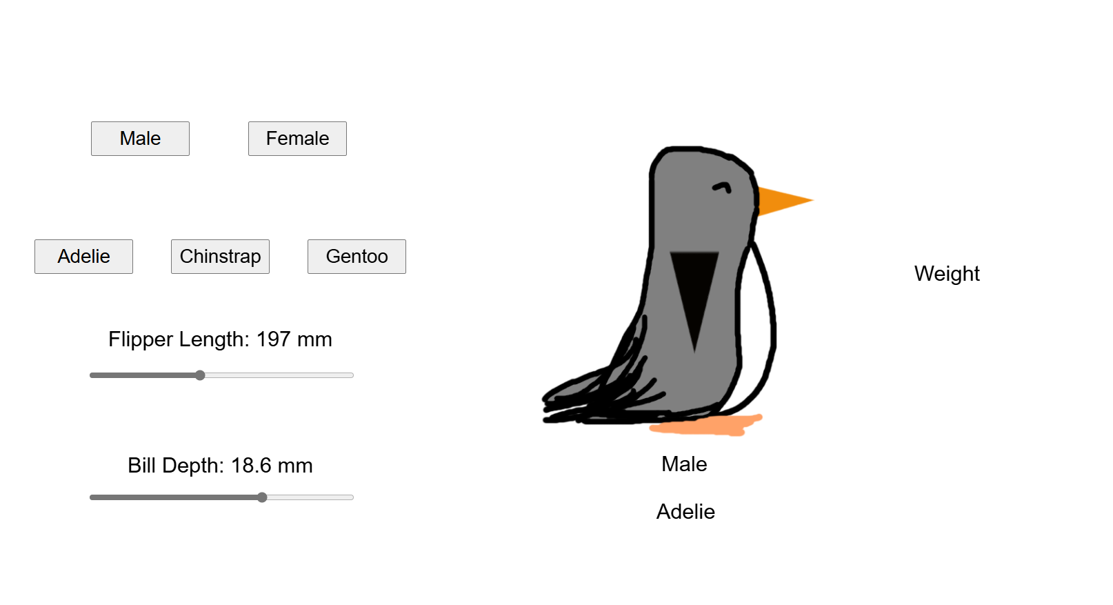
new_data = {'flipper_length_mm': [197], 'sex': ["FEMALE"], 'species': ["Adelie"], 'culmen_depth_mm': [18.6]}
new_penguin = pd.DataFrame(new_data)
model.predict(new_penguin)
Based off our model, we can expect a male gentoo penguin with a 180mm Flipper Length and a 20mm culmen depth to be around 3408.38g.
After all of this review, I worked to take the developed model and use that as the basis for the interactive tool here.